The first type of 2D pattern image created was a tall rectangle aperture. This was generated using the following code:
//tallrectangleThe Fourier transform of the image was then obtained, with the modulus being displayed, through the following code:
nx = 128; ny = 128; //defines the number of elements along x and y
x = linspace(-1,1,nx); //defines the range
y = linspace(-1,1,ny);
[X,Y] = ndgrid(x,y); //creates two 2-D arrays of x and y coordinates
r = X.^2;
r2 = Y.^2; //note element-per-element squaring of X and Y
A = zeros (nx,ny);
A (find(r<0.3) ) = 1;
B = zeros (nx,ny);
B (find(r2<0.05) ) = 1;
C = A.*B;
imshow(C);
imwrite(C,'F:\tallrectangle.bmp');
Igray = imread('F:\AP186 - Activity 6\tallrectangle.bmp');The created image of the tall rectangle aperture and the modulus of its Fourier transform is shown below:
FIgray = fft2(double(Igray));
FSIgray = fftshift(abs(FIgray));
imwrite(uint8(255*abs(FSIgray)/ max(abs(FSIgray))),'F:\AP186 - Activity 6\tallrectangle_FT.bmp');


Fig. 1. Generated tall rectangle aperture image (left) and its FT modulus (right).
The next 2D patterns that were asked were a wide rectangle aperture, two dots along the x-axis which were symmetric about the center, and the same two dots but with different spacing. I also generated a lying rectangle before the wide rectangle since the definition was a bit vague. The respective generating codes used were as follows:
//lyingrectangle
nx = 128; ny = 128; //defines the number of elements along x and y
x = linspace(-1,1,nx); //defines the range
y = linspace(-1,1,ny);
[X,Y] = ndgrid(x,y); //creates two 2-D arrays of x and y coordinates
r = X.^2;
r2 = Y.^2; //note element-per-element squaring of X and Y
A = zeros (nx,ny);
A (find(r<0.05) ) = 1;
B = zeros (nx,ny);
B (find(r2<0.3) ) = 1;
C = A.*B;
imshow(C);
imwrite(C,'F:\lyingrectangle.bmp');
////widerectangle
//nx = 128; ny = 128; //defines the number of elements along x and y
//x = linspace(-1,1,nx); //defines the range
//y = linspace(-1,1,ny);
//[X,Y] = ndgrid(x,y); //creates two 2-D arrays of x and y coordinates
//r = X.^2;
//r2 = Y.^2; //note element-per-element squaring of X and Y
//A = zeros (nx,ny);
//A (find(r<0.3) ) = 1;
//B = zeros (nx,ny);
//B (find(r2<0.7) ) = 1;
//C = A.*B;
//imshow(C);
//imwrite(C,'F:\widerectangle.bmp');
//twodots
nx = 128; ny = 128;
x = linspace(-1,1,nx);
y = linspace(-1,1,ny);
[X,Y] = ndgrid(x,y);
A = zeros (nx,ny);
A(64,48) = 1;
A(64,80) = 1;
imshow(A);
imwrite(A,'F:\twodotspixels.bmp');
//twodots, differentspacingUsing the exact same code used on the tall rectangle aperture image but edited to the filenames of these other 2D pattern images, each Fourier transform modulus was generated in a similar fashion. For each of these patterns, the created image and the modulus of its Fourier transform is shown below:
nx = 128; ny = 128;
x = linspace(-1,1,nx);
y = linspace(-1,1,ny);
[X,Y] = ndgrid(x,y);
A = zeros (nx,ny);
A(64,28) = 1;
A(64,100) = 1;
imshow(A);
imwrite(A,'F:\twodotspixels_diffspacing.bmp');


Fig. 2. Generated images (left) and their respective FT modulus (right).
It can be observed from Fig. 1 that the tall rectangle aperture's FT modulus has a narrow width along the y-axis, which agrees with the expected anamorphic property of such a 2D Fourier transform. Similarly, a rectangle with the exact same dimensions as that tall rectangle but oriented such that it is lying down produces an FT modulus with a narrow width along the x-axis. This can be seen in the first pair of images in Fig. 2.
A wide rectangle produces a very small FT modulus, smaller than that produced by the narrower rectangle. Meanwhile, the two white pixels produce a grating pattern that becomes thinner as the distance between the two white pixels is increased.
For the next part of the activity, the rotation property of Fourier transforms was investigated.
First, the following code was used to create a 2D sinusoid along the x-axis:
//sinusoid along x = corrugated roofThe bias of plus 1 and multiplication by 0.5 was done since sine normally gives values between -1 and 1, so adding 1 would give values between 0 and 2, which would make a multiplication by 0.5 give values between 0 and 1. This range would avoid any clipping that would have occurred from the previous ranges.
nx = 128; ny = 128; //defines the number of elements along x and y
x = linspace(-1,1,nx); //defines the range
y = linspace(-1,1,ny);
[Y,X] = ndgrid(x,y); //creates two 2-D arrays of x and y coordinates
f = 4 //frequency – you may change this later.
theta = 30;
A = 0.5*(sin(2*%pi*f*X)+1); //with bias
imwrite(A,'F:\AP186 - Activity 6\corr_roof.bmp');
Taking the Fourier transform of A and displaying the FT modulus was done using the following code:
Igray = imread('F:\AP186 - Activity 6\corr_roof_wb_6B7_aao.bmp');For frequencies f=4, f=8, and f=16, the following pairs of images were obtained:
FIgray = fft2(double(Igray));
FSIgray = fftshift(abs(FIgray));
imwrite(uint8(255*abs(FSIgray)/ max(abs(FSIgray))),'F:\AP186 - Activity 6\corr_roof_FT.bmp');


Fig. 3. Generated corrugated roofs and their FTs with f = 4, f = 8 and f = 16, respectively.
The FTs in Fig. 3 above seem to consist of three points, one point in the center of the image that is completely white and two points on either side along the x-axis that are gray. These two flanking points are equidistant from the center point. As the frequency was increased, the corrugated roofs decreased in wavelength, and due to anamorphism, this increased the distance between the flanking points and the center point on the FTs.
To test the effect of a rotated sinusoid, the expression for A in the roof-generating code was commented out and a new expression was used:
theta = 30;Generating this newly rotated sinusoid as an image as well as its FT produced the following pair of images:
A = sin(2*%pi*f*(Y*sin(theta) + X*cos(theta)));
A = 0.5*(A+1); //for bias


Fig. 4. Generated images for the corrugated roof rotated by 30 degrees and its FT.
The gray points that flank the white center point in the FT of Fig. 4 move along the new axis of the sinusoid. This seems to be the effect of rotation.
To test the combining of sinusoids and its effect on the obtained FT, the code for A was again commented out and a new code was used, this time giving the product of two corrugated roofs running along the x-axis and the y-axis:
A = sin(2*%pi*4*X).*sin(2*%pi*4*Y);The FT was also obtained, and the pair of images obtained were as follows:

Fig. 5. Generated images for the combined sinusoid and its FT.
The FT produced by the combined sinusoid, as shown in Fig. 5 above, contains five points. The point at the very center of the image is still completely white, while the four points seem like corner points of a small square at the center of the image. This seems to be from the two points flanking the center point being split off into two points at the other axis, signifying a duplication of sorts on the flanking points.
There seems to be a trend of using the previous flanking points produced by FT as the center point of the splitting behavior caused by additional sinusoids.
The next was additional code using the A of the combined sinusoid. Three images were created. For each image, one of the three lines below was added on its own, with the other two commented out. Another image was created by running the code with all three lines present, that is, with none being commented out:
A = A.*sin(2*%pi*f*(Y*sin(15) + X*cos(15)));The images produced and their FTs were as follows:
A = A.*sin(2*%pi*f*(Y*sin(30) + X*cos(30)));
A = A.*sin(2*%pi*f*(Y*sin(45) + X*cos(45)));


Fig. 6. Generated images for the resulting sinusoid and their FT after adding another sinusoid (a) separately with theta of 15 degrees, (b) 30 degrees, (c) 45 degrees, and (d) all of the preceding being added at once.
Note that as more sinusoids are added and more duplication is observed, the brightness of the points become lower and lower. In order to aid for visualization, the black background was replaced with blue for the third column of Fig. 6. It also shows that the gray points are not for one pixel only.
The FT images seem to have points that obtain the characteristics of the added sinusoid. For the first three pairs of images in Fig. 6, the square corner points that were in Fig. 5 are duplicated and displaced in opposite directions along the new axis of the sinusoid upon rotation.
The last pair of images in Fig. 6 show very dim but numerous points which seem to implement all of the duplication and displacement in succession.
For the next part of the activity, more exercises on the convolution theorem were done. Two pixels, separated along the x-axis, were generated. Moreover, the pixels were replaced with circles, and then with squares, and the size was varied for the shapes. The circles were done in Scilab, while the squares were the circle images edited in MS Paint. The Scilab code used was:
nx = 128; ny = 128;The FTs for all of these images were produced.
x = linspace(-1,1,nx);
y = linspace(-1,1,ny);
[Y,X] = ndgrid(x,y);
A = zeros (nx,ny); // for pixels, circles, squares
//twodots, pixels
A(64,48) = 1;
A(64,80) = 1;
//twodots, circles
r = sqrt((X-0.25).^2 + Y.^2);
r2 = sqrt((X+0.25).^2 + Y.^2);
A (find(r<0.03125)) = 1; // r in pixels = 64*r
A (find(r2<0.03125)) = 1; // r2 in pixels = 64*r2


Fig. 7. Generated images and FTs of two pixels, two circle with radius of 2, 4, and 8 pixels, and two squares with side length of 4, 8, and 16 pixels.
As observed from Fig. 7, the circular shape was present in the FT of the circles, and the square shape was also present in the FT of the squares. There was also a common black and white fringe pattern with same length per fringe across all FTs in Fig. 7, which means that it was dictated by the location of the pair of shapes. As for the anamorphic property of FT, it is seen once again with the increase in shape size causing a smaller shape on the FT.
The squares were then replaced with Gaussians. This was done using the following code:
//twodots, gaussiansThe peak location mu_naught was kept constant since it was where the dots originally were. Meanwhile, the sigma was varied to create different Gaussian images, and the FTs were obtained for those images. For sigma = 0.025, 0.05, and 0.1, the following pairs of images were produced:
mu_naught = 0.25; //peak location
sigma = 0.025;
A1 = exp(-(((X+mu_naught).^2)+Y.^2)/(sigma^2));
A2 = exp(-(((X-mu_naught).^2)+Y.^2)/(sigma^2));
A = A1 + A2;
imshow(A);
imwrite(A,'E:\AP186 - Activity 6\gaussians_s=0.025.bmp');
Igray = imread('E:\AP186 - Activity 6\gaussians_s=0.025.bmp');
FIgray = fft2(double(Igray));
FSIgray = fftshift(abs(FIgray));
imwrite(uint8(255*abs(FSIgray)/ max(abs(FSIgray))),'E:\AP186 - Activity 6\gaussians_s=0.025_FT.bmp');


Fig. 8. Generated Gaussian images and their FTs for sigma = 0.025, 0.05, and 0.1.
Compared to the circles, the FTs produced by Gaussians no longer have the surrounding patterns. Meanwhile, anamorphism is still observed, since an increase in sigma creates larger Gaussians, which in turn produce smaller FT patterns.
After this, an image representing a 200 by 200 array of zeros was created using MS Paint. This is basically a black image with 200 by 200 pixels in dimension. Random ones were added to the image by arbitrarily placing white pixels across the image. This was then saved as '10random1s.bmp'.
A 3 by 3 pattern that looked like a small white letter 'x' on a black background was created in MS Paint. Upon producing this other image, with filename of '3x3pattern,bmp', the two were read in Scilab and convolved. The code used is shown below:
A = imread('E:\AP186 - Activity 6\10random1s.bmp');The images produced were as follows:
d = imread('E:\AP186 - Activity 6\3x3pattern.bmp');
cAd = conv2(double(A),double(d));
imshow(cAd);
imwrite(cAd,'E:\AP186 - Activity 6\10random1s_conv.bmp')


Fig. 9. Generated image of randomly placed ones in an array of zeros before and after convolving with a small 3 by 3 pattern that looked like a small white letter 'x' on a black background.
It can be seen that convolving gave the characteristics of the small pattern onto the white pixel dots, which approximate Dirac deltas, of the other image, producing the latter image in Fig. 9.
White pixel dots approximating Dirac deltas were placed in another array of zeros, but this time, Scilab was used to create the image. The dots were spaced evenly across the x-axis and the y-axis of the array. This spacing was edited from 4 pixels, 8 pixels, and then 20 pixels between dots. The FTs were then obtained. All of this was done using the following code:
nx = 200; ny = 200;The obtained images and their FTs are shown below:
A = zeros (nx,ny);
s = 20; // spacing between axis dots
for i=1:200
if modulo(i,s) == 0 then
A(100,i) = 1;
A(i,100) = 1;
end
end
imshow(A);
imwrite(A,'E:\AP186 - Activity 6\axisdots_s=20.bmp');
Igray = imread('E:\AP186 - Activity 6\axisdots_s=20.bmp');
FIgray = fft2(double(Igray));
FSIgray = fftshift(abs(FIgray));
imwrite(uint8(255*abs(FSIgray)/ max(abs(FSIgray))),'E:\AP186 - Activity 6\axisdots_s=20_FT.bmp');


Fig. 10. Generated images of dots spaced every 4 pixels, 8 pixels, and 20 pixels across the axes and their FTs.
The FTs produced were horizontal and vertical white lines crisscrossing each other. The number of black squares formed correspond to the pixel spacing of the dots, with four black squares per side for dots that are spaced at every four pixels, eight squares per side for eight pixel spacing, and twenty squares for twenty pixel spacing. This follows anamorphic property of FT since the larger spacing between dots causes a smaller spacing between white lines on the FT images.
For the next part of the activity, ridge enhancement of fingerprints was done. I was able to scan my own fingerprint marked using a stamp pad on a clean white sheet of paper. I then opened it using Scilab, took the grayscale value of this image, took its FT, and saved it under a different filename. These steps were done using the following code:
f0 = imread('E:\AP186 - Activity 6\fingerprint2.png');This then gave me a chance to look at the FT and see which parts should be masked. The fingerprint in grayscale as well as the obtained FT are as follows:
f = rgb2gray(f0);
FIgray = fft2(double(f));
imwrite(uint8(255*log(abs(fftshift(FIgray)))/max(log(abs(fftshift(FIgray))))),'E:\AP186 - Activity 6\fingerprint_FT.bmp');

Fig. 11. Scanned image of my fingerprint in grayscale.

Fig. 12. The FT of the scanned image of my fingerprint.
The prominent ring as well as the very center of the FT should be white for the mask, while everywhere else is presumably noise and does not contribute to the fingerprint ridge pattern. This was what I followed in creating the following filter mask in MS Paint:


Fig. 13. The filter mask I created (right) compared with the FT of the fingerprint (left).
The mask was applied through element by element multiplication of the arrays produced from reading the mask image and the fingerprint image. To obtain the properly oriented post-mask fingerprint image, FT was done three times. These steps are illustrated in the following code:
f0 = imread('E:\AP186 - Activity 6\fingerprint2.png');The obtained post-mask fingerprint image is as follows:
f = rgb2gray(f0);
mask = fftshift(double(imread('E:\AP186 - Activity 6\mask.bmp')));
FIgray = fft2(double(f));
FIgray = FIgray.*mask;
f_I = fft2(fft2(fft2(FIgray)));
imshow(uint8(255*(abs(f_I))/max(abs(f_I))));
imwrite(uint8(255*(abs(f_I))/max(abs(f_I))),'E:\AP186 - Activity 6\fingerprint_postmask.bmp');


Fig. 14. The obtained post-mask fingerprint image (right) compared with the original (left).
As can be seen in Fig. 14, the blotches of the original fingerprint image were reduced to discolorations in the post-mask fingerprint image, revealing the ridge patterns underneath.
For the next part of the activity, line removal was done on scanned pictures of the lunar landing that were provided to us by our instructor, Ma'am Jing Soriano. A very similar process as the previous part was done, as can be seen in the similarity of code used:
lunar = imread('E:\AP186 - Activity 6\Lunar Orbiter Image with Lines.jpg');The lunar landing image used and the FT of it that I obtained were as follows:
flunar = fft2(double(lunar));
sflunar = fftshift(flunar);
imwrite(uint8(255*log(abs(sflunar))/max(log(abs(sflunar)))),'E:\AP186 - Activity 6\lunar_FFT.bmp');
mask = fftshift(double(imread('E:\AP186 - Activity 6\lunar_mask.bmp')));
flunar = flunar.*mask;
clunar = fft2(fft2(fft2(flunar)));
imshow(uint8(255*(abs(clunar))/max(abs(clunar))));
imwrite(uint8(255*(abs(clunar))/max(abs(clunar))),'E:\AP186 - Activity 6\lunar_cleaned.bmp');

Fig. 15. Scanned lunar landing image provided to us by Ma'am Jing.

Fig. 16. The FT of the scanned lunar landing image.
The mask I used aimed to get all of the information except for the cause of the scan lines, which, similar to the dots in Fig. 10, are at the y-axis on the FT image. This led me to create the following filter mask, making sure that there is one white pixel at the very center of the mask image:


Fig. 17. The filter mask I created (right) compared with the FT of the lunar image (left).
The obtained post-mask lunar landing image is as follows:


Fig. 18. The obtained lunar landing image cleaned of lines (right) compared with the original (left).
The above further illustrates the remarkable ability of filter masks based on FT to remove undesired parts of an image. This part of the activity was the one that impressed me the most and made me feel accomplished for doing, due to how nice the resulting image turned out.
For the last part of the activity, the removal of a painting's canvas weave as well as modelling of that same canvas weave was done. A very similar process was done as with the previous two parts of the activity. This is once again evident in the code I used, shown below:
painting = rgb2gray(imread('E:\AP186 - Activity 6\cropped_painting2.jpg'));The original image provided to us by Ma'am Jing was too large when I try to read it in Scilab, which is why I decided to crop it to only cover a smaller portion of the painting. I also saved a grayscale version of this cropped image, since the rgb2gray() in the above code uses the grayscale version.
fpainting = fft2(double(painting));
sfpainting = fftshift(fpainting);
imwrite(uint8(255*log(abs(sfpainting))/max(log(abs(sfpainting)))),'E:\AP186 - Activity 6\painting_FT.bmp');
mask = fftshift(double(imread('E:\AP186 - Activity 6\painting_mask5.bmp')));
fpainting = fpainting.*mask;
cpainting = fft2(fft2(fft2(fpainting)));
imwrite(uint8(255*(abs(cpainting))/max(abs(cpainting))),'E:\AP186 - Activity 6\painting_grayscale_cleaned5.bmp');

Fig. 19. The original painting image provided to us by Ma'am Jing.


Fig. 20. Cropped image of the painting and its grayscale version.
The cropped grayscale image in Fig. 20 was the image I used in order to take the FT, as shown below:

Fig. 21. The obtained FT of the cropped grayscale painting image.
I then created various filter masks based on this FT. The inverse of these filter masks also give the part of the painting being removed, which would effectively model the canvas weave pattern. The quality of the filter mask dictates how much detail is removed as the canvas weave pattern is removed.
The filter masks I used were the following:


Fig. 22. Various filter masks created for the painting and canvas weave.
Using each of these filter masks on the cropped grayscale painting produced the following results:

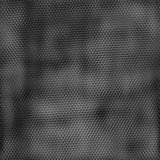


Fig. 23. The respective cleaned paintings and canvas weaves that were generated from the filter masks.
From Fig. 23, it can be seen that too large masking shapes on the FT cause more detail to be lost from the painting. The simulated canvas weave show just how much detail was also being lost, with the second and third pair of images having almost a blurred copy of the painting on the canvas weave. Although those same pairs seem to have cleaned paintings that had less remnants of the canvas weave, the loss of detail is still undesirable.
My first try was the first pair of images, and this pair seemed to still have noticeable canvas weave on the cleaned image, as well as traces of the original painting on the simulated canvas weave. The last attempt I settled on was the fourth pair of images, with the least amount of original painting traces on the simulated canvas weave.
This was a very long activity, and the making of the blog proved to be very overwhelming as a task. I think that making the blog little by little helped in eventually finishing it, since there were just so many images that were produced. Still, this is the point of the course at which I got really, really impressed with the applications. Seeing just how applicable these skills we were learning were made me happy. In that regard, I would like to thank Robbie Esperanza and Zed Fernandez for helping me throughout the activity, especially with the masking parts of the activity.
Self-Evaluation: 9/10